Abstract
The Hierarchical Genetic Algorithms (HGA) are a kind of Genetic Algorithms (GA) applicable to solve hierarchical problems.
Table of Contents
1. Definition↑
The Hierarchical Genetic Algorithms (HGA) were developed to solve a particular class of hierarchical problems: the tree to build refers to the set theory. In fact, HGA are a genetic framework for placement problems, i.e. each particular problem needs its own customization. As the name suggests, HGA are an extension of the conventional Genetic Algorithms.
Starting from a set of objects,
2. Encoding↑
In the HGA, the chromosomes represents a given tree. The coding scheme includes a node element and an object element. In practice, each chromosomes is represented by:
- An array of nodes, each node containing the index of the first child node and the number of its child node.
- An array holds the assignation of each object.
Figure 1 proposes an example of a tree defining \(6\) nodes of \(9\) objects.
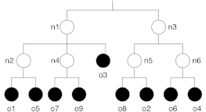
Figure 1. Example of a tree.
The corresponding chromosome is presented at Figure 2. The “left part” of the chromosome represents the description of the hierarchy of nodes. The array begins with the two top nodes (\(n_1\) and \(n_3\)). Each class is described as a pair of (index,length). For example, \(n_1\) is defined by \((2,2)\) since the index of the first sub-node (\(n_2\)) is \(1\) and it has two child nodes (\(n_2\) and \(n_4\)). The “right part” of the chromosome represents the assignment of the different object. For example, object \(o_5\) is assigned to \(n_6\).
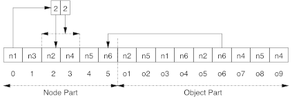
Figure 2. Example of a chromosome.
3. Evaluation↑
The evaluation of the chromosomes is an important feature of a genetic algorithm. Since the goal is to obtain a balanced tree, an idea is to minimize the average length of the path to reach each object.
To compute the length of a given path, I propose to sum the depth of the path (the number of nodes to traverse) with the number of choices at each intermediate node. Let us define \(n_{n}(j)\) as the number of child nodes of \(n_j\) (\(n_{n}(root)\) is the number of top nodes) and \(n_{o}(j)\) as the number of objects assigned to node \(n_j\). Moreover, let us define a cost, \(cost(n_{j})\), for each node, \(n_j\):
\[cost(n_{j})=\left\{ \begin{array}{lc} n_{n}(root) & Parent(n_{j})=root\\ cost(Parent(n_{j}))+n_{n}(Parent(n_{j}))+n_{o}(Parent(n_{j})) & Parent(n_{j})\neq root \end{array}\right.\]
where \(Parent(n_{j})\) is a function returning the parent node of \(n_j\) and \(root\) is the root node.
The cost function, \(cost\), to minimize is defined as:
\[cost=\frac{1}{|\mathcal{O}|}\sum_{i}cost(Assign(o_{i}))\]
where \(Assign(o_{i})\) is a function returning the node where object \(o_i\) is assigned. Figures 3 and 4 show two tree examples. When comparing \(T_1\) and \(T_2\), it seems clear that \(T_2\) is more unbalanced than \(T_1\).
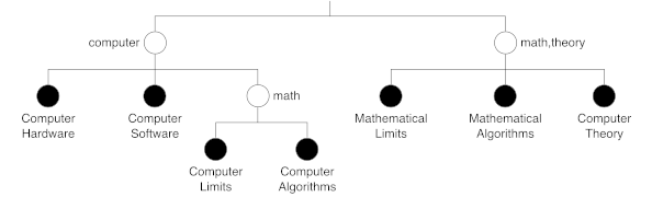
Figure 3. Tree T1.
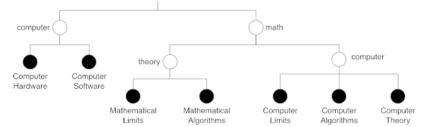
Figure 4. Tree T2.
Let us compute the cost function for these trees:
\begin{align}cost(T_{1})&=&\frac{6+6+9+9+5+5+5}{7}=6.43\\cost(T_{2})&=&\frac{8+8+9+9+9+5+5}{7}=7.57\end{align}
As expected, \(cost(T_{2})>cost(T_{1})\).
4. Heuristic↑
Since the GA are meta-heuristics, the heuristics play an important role and must be adapted for the particularity of the problem. This section presents the heuristic used by the HGA. Algorithm 1 shows the generic idea : the objects are randomly selected and a node in the tree is searched that can hold the current object.
Require:
Tree \(T\)
Build a random array of unassigned objects of \(T\), \(\mathcal{O}\)
for (\(\forall o_{i}\in\mathcal{O}\)):
\(New\leftarrow Find(T,o_{i})\)
\(T.Attach(New,o_{i})\)
Algorithm 1. The heuristic, Heuristc(T).
Algorithm 2 describes the method that searches for a node that will hold an object (\(Attr\) is a function returning the list of attributes of an object or a node). The basic idea is to find the “first highest” node that can hold a given object. The method parses each level in the hierarchy to find a node that can hold a given object. To be selected, a node must share at least one attribute with the object. Three situation may occur:
- The node has exactly the same attributes as the object : The object will be attached to it.
- All the attributes of the node are attributes of the object : The method looks further in the branch of the tree corresponding to it.
- Some attributes of the node are attributes of the object : an intermediate node with the common attributes must be created.
Of course, if no node shares some attributes with the object, a new root node must be created.
Require:
Object \(o\) to assigned and a tree \(T\)
\(Parent\leftarrow0\) {Start at the root node}
loop:
Build a random array containing all the child nodes of \(Parent\), \(N\)
\(GoDeeper\leftarrow\mathrm{False}\)
\(None\leftarrow0\)
\(NbMax\leftarrow0\)
for (\(\forall n_{i}\in\mathcal{N}\)):
\(Nb\leftarrow|Attr(o)\cup Attr(n_{i})|\)
if (\(Nb=0\)):
continue
if (\(Nb=|Attr(n_{i})|\)): {Good branch was found}
if (\(Nb=|Attr(o)|\)):
return ni
\(Parent\leftarrow n_{i}\)
\(GoDeeper\leftarrow\mathrm{True}\)
break
if (\(NbMax<Nb\)):
\(NbMax\leftarrow Nb\)
\(Node\leftarrow n_{i}\)
if (\(GoDeeper=\mathrm{True}\)):
break
if (\(Node=0\)):
return \(T.NewNode(Attr(o),Parent)\)
{\(Node\) contains some attributes not representing the object.}
\(Common=Attr(o)\cup Attr(Node)\)
if (\(Parent\) and \(|Attr(Parent)|=|Common|\)):
return\(T.NewNode(Attr(o),Parent)\)
\(New\leftarrow T.NewNode(Common,Parent)\) {Create a new node attached to \(Parent\)}
\(T.MoveNode(New,Node)\) {\(New\) has \(Node\) as child}
return \(T.NewNode(Common,New)\) {\(New\) has a new node containing the object}
Algorithm 2. Find a node for object o, Find(o,T).
5. Crossover↑
The role of the crossover operator is to construct a new chromosome using two parents. If the operator mix “good patterns” from both parents, the child chromosome should be a “good” one.
The crossover proposed for the HGA combines the trees of both parent based on a crossing site defined as two nodes (one in each parent) having the same attributes. It is then possible to replace the branch of one tree with the other.
In practice, the operator verifies that an object is not assigned twice and run the heuristic if there remains unassigned objects. Algorithm 3 describes the crossover operator ((Objs) is a function returning the list of objects attached to a node).
Require:
Two parent trees, \(T_1\) and \(T_2\), and a child tree, \(C\)
Build a random array containing all the nodes of \(T_1\), \(\mathcal{N}_{1}\)
Build a random array containing all the nodes of \(T_2\), \(\mathcal{N}_{2}\)
\(Node_{1}\leftarrow 0\)
\(Node_{2}\leftarrow 0\)
for (\(\forall n_{j}\in\mathcal{N}_{1}\)):
for (\(\forall n_{k}\in\mathcal{N}_{2}\)):
if (\(Attr(n_{j})=Attr(n_{k})\)):
\(Node_{1}\leftarrow n_{j}\)
\(Node_{2}\leftarrow n_{k}\)
break
if (\(Node_{1}\neq0\)):
\(Clear(C)\)
\(thObjs\leftarrow Objs(Node_{2})\)
\(Node\leftarrow C.CopyExceptBranchAndObjects(T_{1},Node_{1},thObjs)\)
\(New\leftarrow C.ReserveNode()\)
\(C.Insert(Node,New)\)
\(C.CopyExceptBranch(Node_{2})\)
\(Heuristic(C)\)
else:
print “Error: no crossing site”
Algorithm 3. Crossover of the HGA
An important element is that, if a crossing site is not found (there are not two nodes with the same attributes from each tree), the crossover cannot be done.
6. Mutation↑
Te role of the mutation operator is modify a given chromosome to explore new portions of the search space. Most of the time, it is implemented as a little modification of the chromosome. I apply this idea by choosing randomly a node and delete it, and using then the heuristic to attach the unassigned objects (Algorithm 4).
Require:
Tree \(T\)
Choose randomly a node, \(Node\)
\(T.Delete(Node)\)
\(Heuristic(T)\)
Algorithm 4. Mutation of the HGA
7. Inversion↑
The inversion, whose role consists in presenting differently a given chromosome without changing its corresponding information, is not implemented in the HGA, because all the operators are based on the “interpretation” of the chromosomes rather than on the encoding of the chromosomes.