2D Genetic Algorithms

The 2D Genetic Algorithms (2D-GA) were developed to solve placement problems. In fact, 2D-GA are a genetic framework for placement problems, i.e. each particular problem needs its own customization. As the name suggests, 2D-GA are an extension of the conventional Genetic Algorithms.

2. Encoding↑

Remember that for the placement problems, each object may have multiple valid orientations. The solution consists of a position for each object with a given valid orientation. Figure 1 proposes two solutions, \(C_1\) and \(C_2\) for a placement problem.

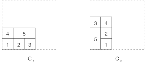
Figure 1. Two solutions for a placement problem.

In the 2D-GA, the chromosomes store for the different object of a solution their position and the particular orientation used for the placement. Figure 1 shows two examples for which the corresponding chromosomes are:

\[C_{1}={(0,0,Normal),(10,0,Normal),(20,0,Normal),(0,10,Normal)(10,10,Normal)}\]

\[C_{2}={(10,0,Normal),(10,10,Normal),(0,20,Normal),(20,20,Normal)(0,0,Rota90)}\]

3. Evaluation↑

A genetic algorithm needs to evaluate the chromosomes of a population. For the 2D-GA, the performance of a particular chromosome (placement) is determined by two criteria that are difficult to compare:

Area Criterion. The total area occupied by the elements.
Distance criterion. The sum of the nets distances.

The evaluation of a given placement is thus a multi-criteria problem, and we decide to use the multiple objective approach based on the PROMETHEE method. Actually, the two criteria have the same characteristics and are both to be minimized:

a weight of 1;
a preference’s threshold of 0.2;
an indifference’s threshold of 0.05;

It is possible to change the values of the PROMETHEE parameters for a specific problem¹.

4. Heuristics↑

Because GA are meta-heuristic, heuristics are central in the 2D-GA. Three different heuristics were developed based on a same generic approach described by Algorithm 1.

Require:

Objects to place, \(O\)

Build a random array of not placed objects, \(O\)

while (\(∃o_i∈O\)):

\(o_i←MostConnected(O)\)

\((x,y)←IsFreeSpace(o_i)\)

if \((x,y)\) are not valid:

\((x,y)←PlaceRect(oi)LocalOptimization(o_i)\)

\(UpdateFreeSpace()\)

Algorithm 1. Generic placement heuristic.

For all the objects to place, the heuristic selects iteratively the most connected one (section 4.1) and look if an existing free space can hold it. If no, a method place the object, and a local optimization is performed (section 4.2). Finally, the free spaces are updated. Sections 4.3, 4.4 and 4.5 presents three strategies to place an object. Section 4.6 explains the free space problem.

4.1. Select Object to Place↑

When choosing a object to place, each heuristic parses the random array of object \(O\). For each object, the heuristic computes the sum of the weights of the connections involving it and which are composed from at least one already placed object.

This method ensures that the most connected objects are placed first, while the randomization of the array of objects to place should provide diversity in the population.

4.2. Local Optimization↑

To increase the speed of the implemented heuristics, the objects are first considered as rectangles (the bounding rectangles of the corresponding polygons). Once the rectangle is placed, the position must be adapted by transforming it into the original polygon. This is the role of the local optimization. Figure 2 shows two examples, where the object \(2\) is first placed as a rectangle.

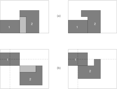
Figure 2. The local optimization.

In the first example (a), the object must be placed as close as possible from the “bottom-left” corner, while in the second example (b), it must be placed as close as possible from the point represented by the intersection of the dashed lines.

4.3. Bottom-Left Heuristic↑

The bottom-left heuristic is a very simple method. The basic principle is to place the first object in the bottom-left corner. The next objects are placed next to it at the right until the horizontal limit is exceeded. After that, the heuristic creates a “new line”, i.e. starts for the next objects again from the left limit and at a given height determined by the highest object already placed. Figure 3 shows an example of this heuristic (the numbers indicate the order in which the objects were placed).

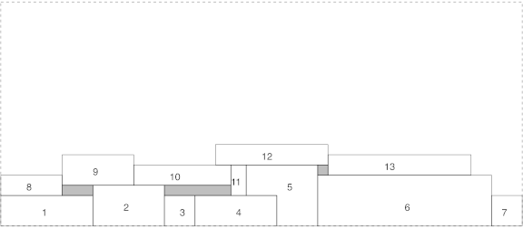
Figure 3. The bottom-left heuristic.

While this heuristic is very simple, efficient and fast, it has a big drawback: the bounding rectangle will have a length close to the one of the horizontal limit, but the height can be much smaller than the vertical limit. For some problems where the resulting rectangle has to be “balanced”, this heuristic does not provide good results. Another problem is that two consecutively placed objects, which are connected together, are not necessary place close from each other (objects \(7\) and \(8\) of Figure 3), this is also a disadvantage for the “distance” criterion.

4.4. Edge Heuristic↑

The edge heuristic is derived from the bottom-left, with the aim to obtain a bounding rectangle whose dimensions are proportional to the limits of the problem. The first object is also put in the bottom-left corner, but for the second object, the heuristic determines two different positions: at the right of the first object or above it. For these positions, the heuristic computes the rate heightlength to determine the position which gives the closest rate to the corresponding one of the limiting height and length. The next objects are treated in the same way. Figure 4 shows an example of this heuristic (the numbers indicate the order in which the objects were placed).

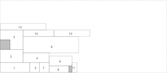
Figure 4. The edge heuristic.

With this heuristic, the problem of the bounding rectangle of the bottom-left heuristic is solved. The price to pay is that the total area of the bounding rectangle is larger than the one obtain with the bottom-left heuristic. It works a little bit slower than the bottom-left heuristic. It also has the same problem than the bottom-left heuristic one in regards of the “distance” criterion, because again two consecutive objects can be placed far from each other.

4.5. The Center Heuristic↑

To avoid the problem of the “distance” criterion, the center heuristic was developed. The idea is to place the objects as close as possible from the center. Of course, when the number of objects already placed increases, the number of possible positions for the next object also increases. The result is that this method is really slower than the other two. Figure 5 shows an example of this approach (the numbers indicate the order in which the objects were placed).

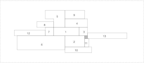
Figure 5. The center heuristic.

This heuristic gives the best results in terms of “distance” criterion while it still give performing solutions in terms of “area” criterion.

4.6. Free Space Problem↑

One of the problem which appears when placing objects, in particular if they are polygons, is the formation of “free spaces”, i.e. regions without objects completely enclosed by objects and that could not be used directly by the heuristics. Figure 6 shows an example (the numbers represent again the order in which the objects were placed).

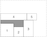
Figure 6. The free space problem.

When the object \(4\) is placed, it automatically creates a “free space”, a region colored in gray. It is also evident that the object \(5\) can be placed in this “free space”. This is why a method was developed to compute the polygons corresponding to these “free spaces” after each positioning. Before the algorithm determines possible positions according the heuristic strategy, it looks whether there is a “free space” that can hold this element.

The problem of finding a good “free space” for a given element is close to the “dynamic storage allocation” problem. When a program is asking for a given quantity of memory, the operating system must choose between the free regions in RAM, which one to be used for the given bloc, in order to limit the fragmentation of the memory (Figure 7).

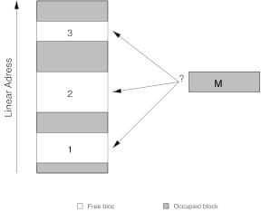
Figure 7. The dynamic storage allocation.

There are several algorithms to solve this problem [1]:

First-fit. The first region that can hold the bloc is chosen (bloc \(M\) in bloc \(1\)).
Best-fit. The smallest region than can hold the bloc is chosen (bloc \(M\) in bloc \(3\)).
Worst-fit. The largest region than can hold the bloc is chosen (bloc \(M\) in bloc \(2\)).

These methods were compared, in particular in [2] and [3], where it was demonstrated that the first-fit and best-fit strategies are better than the worst-fit. For many years, the best-fit was applied because it preserves the larger free regions for future demands of big quantities of memory. On the other hand, it increases the number of very few regions that will never hold a bloc. In fact, the first-fit and best-fit strategies give, in terms of memory fragmentation, the same kind of quality. That is the reason why, the first-fit is used because it is faster than the best-fit where all the free region have to be controlled.

In the case of the “free spaces” treatment, a first-fit strategy was implemented: the first “free space” that can hold a given element is chosen.

5. Initialization↑

Once the coding has been defined, the 2D-GA must initialize the population. The method used depends on the particular problem because the different solutions must satisfy the hard constraints. In practice, a heuristic should be defined to place a given set of objects.

6. Crossover↑

The role of the crossover is to construct a new solution called a child by taking “good” portions of two solutions called the parents. In the case of placement problems, an intuitive crossover is to select a portion of the placement of both parents as the basis to construct the children.

Figure 8. The crossover operator for the 2D-GA.

An example is showed at Figure 8. From each parent, a set of objects are chosen (filled in gray on the figure), one child is further constructed by using these sets.

6.1. Object Selection↑

The crossover depends of course of the choice of the objects to be inherited from the parents. A good set of objects is characterized by two criteria:

the selected objects must be placed close together;
the selected objects must be ”well connected”.

The selector first classify all the objects by “well connected”. To define a “well connected” object, we reach two criteria:

Weight Criterion. The sum of the weights of the nets involving the object.
Distance Criterion. The sum of the net’s distances involving the object.

This is a multi-criteria problem, and the PROMETHEE method is used to solve it. The two criteria have the same characteristics:

a weight of 1;
a preference’s threshold of 0.2;
an indifference’s threshold of 0.05;

Of course, the “weight criterion” has to be maximized and the “distance criterion” has to be minimized².

The selector chooses the “best connected” object not already selected ². After that, the selector looks which is the second “best connected” object not already selected so that the two objects can be contained in the “choice rectangle” whose size is the quarter of the total occupied space by all the objects. The set of selected objects is filled with these two objects, and all the other objects that are inside the “choice rectangle”.

An example is showed at Figure 9, where object \(1\) is the “best connected” and object \(2\) is the second “best connected”, and the “choice rectangle” is drawn as dashed. The selected objects are those in gray.

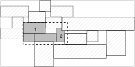
Figure 9. The object selection.

6.2. Child Construction↑

To construct a child, the operator considers that the sets of objects of the two parents are a sort of super blocs that can be treated by the heuristics as single objects. Then a heuristic is used to place these two objects and all the others that are not selected in one of the parent sets.

7. Mutation↑

The strategy of the mutation currently implemented is to create a totally new chromosome by using a heuristics.

Of course, this strategy limits the advantages of the way the mutation choose the chromosomes, that is the reason why developing a new mutation strategy will be one of the priorities in the future developments.

8. Inversion↑

The inversion, whose role consists in presenting differently a given chromosome without changing its corresponding information, is not implemented in the 2D-GA, because all the operators are based on the “interpretation” of the chromosomes rather than on the encoding of the chromosomes.

9. Validation↑

A first prototype was developed during a research project aimed to develop a method of helping to create Very-Large-Scale Integration (VLSI) chips, and funded by the Walloon Region from 1999 to 2001. Furthermore, because not enough tests have being done actually, it is only possible to present qualitative results rather than quantitative ones.

For the VLSI problem, where the connections are a very important aspect, the best placement strategy is the center heuristic, because it guarantees that two objects treated consecutively will be placed closed from each other. Furthermore, if the external connectors are disposed around the limiting area, the objects can be place at “equal” distance from each border. An example is showed at Figure 10. With the bottom-left and edge heuristics, all the elements placed will be translated to the bottom-left corner (Position \(O\)), which implies an amelioration for the net \(a\), but a deterioration for all other nets represented.

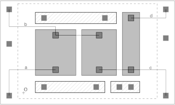
Figure 10. Advantages of the “center” heuristic.

For the crossover, a problem occurs when there are some large blocs in comparison to the limiting area. An example is showed at Figure 11, where the two best objects (\(1\) and \(2\)), selected during the crossover, define a rectangle that holds only a single object. In this case, no interesting information are shared, because the crossover is reduced to run the initial heuristic. This problem becomes important when there are only a few “big” objects to place.

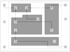
Figure 11. Problem for the element selection in the crossover operator.

References↑

[1] Donald E. Knuth, The Art of Computer Programming, Vol. 1: Fundamental Algorithms, 2ᵉ ed., Addison-Wesley, 1998.

[2] Carter Bays, “A Comparaison of Next-Fit, First-Fit, and Best-Fit”, Communications of the ACM, 20(3), pp. 191—192, 1977.

[3] John E. Shore, “On the External Fragmentation Produced by First-Fit and Best-Fit Allocation Strategies”, Communications of the ACM, 18(8), pp. 443—440,1975.

Notes↑

It is also possible to change the value during the evolution process, but there are actually no reasons to implement something like this. ↩︎
It is possible to change the values of the PROMETHEE parameters for a specific problem. ↩︎
In fact, the same object cannot be selected in both parent, i.e. when an object is chosen in one parent, it cannot be chosen in the second parent. ↩︎

Abstract

Table of Contents

1. Definition↑